Excel Tip: Clear / Unfilter FILTERs Quickly

In Order to Clear / Unfilter a filter quickly you can use the Filter Hotkey Two Times :

Press 2 Times : CTRL + SHIFT + L 

Created by DoMyExcel.com © | Excel & VBA Consulting | Customized Excel Solutions starting at 29 USD

Services provided to Individuals and Businesses | Free Quote: DoMyExcel@gmail.com

How to select all the pictures of a worksheet in EXCEL

To select all the shapes / objects / pictures of a worksheet in EXCEL, simply select one of the shapes and press "CTRL"+ A. You can then copy them, delete them all, etc.

Created by DoMyExcel.com © | Excel & VBA Consulting | Customized Excel Solutions starting at 29 USD

Services provided to Individuals and Businesses | Free Quote: DoMyExcel@gmail.com

How to receive an text input from a message box in EXCEL VBA

If you want to ask the user for an input, you can create a userform or you can simply use the Inputbox() method of VBA. For example:

a = InputBox("Enter the name of the picture")

Created by DoMyExcel.com © | Excel & VBA Consulting | Customized Excel Solutions starting at 29 USD

Services provided to Individuals and Businesses | Free Quote: DoMyExcel@gmail.com

How to highlight an option button in EXCEL when it is selected by the user (no macro needed)

If you want to highlight the selected option button for your custom form in EXCEL, first set the background of the option button as "Transparent": Right click on the option button > "Format Control..." then on tab "Colors and Lines, put the "Transparency" level at 100% and press "OK":

Then if the result of your option button appear in cell "A5" for example (see previous post here to see how to do) then in cell A1 and A2 (behind the option buttons), enter respectivelly the following formulas:

"=if(A5=1,"color","")"

"=if(A5=2,"color","")"

Finally, create a conditional format to color the cell when the value of the cell is equal to "color". 

Trick to not show the formula: put the default font color of A1 and A2 as white and in the conditional formating options, set the font color to be same as the cell background color when the value is equal to "color".

As a result, the option button will be highlighted once the user select it:

Created by DoMyExcel.com © | Excel & VBA Consulting | Customized Excel Solutions starting at 29 USD

Services provided to Individuals and Businesses | Free Quote: DoMyExcel@gmail.com

How to make a user friendly filter for a pivot table in EXCEL using slicer

Since EXCEL 2007, there is a function called "Slicer" that permits to have a better user experience when it comes to filtering data in a pivot table. 
Example on below pivot table:

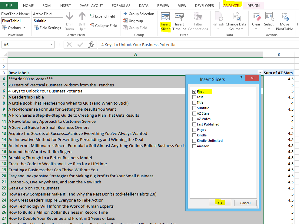
Instead of putting another entry in the "Filters" section of the pivot table, select the pivot table and press "Insert Slicer" in the "Analyze" tab. Then check out the field you want to filter:

As a result you will have a user friendly menu where you can easily search for the name you want to filter and select multiple entry to sort out at once:

Created by DoMyExcel.com © | Excel & VBA Consulting | Customized Excel Solutions starting at 29 USD

Services provided to Individuals and Businesses | Free Quote: DoMyExcel@gmail.com

Excel Tip: Write and Edit Formulas in several sheets at the same time!

You can Edit several Worksheets in Excel at the same time just by Selecting multiple Sheet Tabs through holding the SHIFT button. 

After the Sheets are selected you can keep on editing them until you click in one specific WorkSheet again.

The selection of Sheets can be used to input formulas and to edit the format of cells.

Created by DoMyExcel.com © | Excel & VBA Consulting | Customized Excel Solutions starting at 29 USD

Services provided to Individuals and Businesses | Free Quote: DoMyExcel@gmail.com

Good practice when using EXCEL comparison function (VLOOKUP(), MATCH(), INDEX()) of values in text and number format

The "TRIM()" function in EXCEL helps to prevent error when comparing values in number format with value in text format. This "TRIM()" function will remove all the "space characters: in front of the value and will also convert any number format into a text format.
 



 

This function is particularly interesting when a large number of data need to be compared. It will ensure that you are comparing correctly text to text.

 

One of the good practice is therefore to add one more column to trim the keys of your database, and then to search the trimmed value into this column (works also with MATCH() function, INDEX() function, etc.)

 

 

Created by DoMyExcel.com © | Excel & VBA Consulting | Customized Excel Solutions starting at 29 USD

Services provided to Individuals and Businesses | Free Quote: DoMyExcel@gmail.com

How to remove the hyperlinks from selected range in EXCEL

There is a built in function in EXCEL to remove the hyperlinks: Select the designated area and go to "Home" ribbon > "Clear" dropdown menu > and press "Clear Hyperlinks" :
 

 

 

Created by DoMyExcel.com © | Excel & VBA Consulting | Customized Excel Solutions starting at 29 USD

Services provided to Individuals and Businesses | Free Quote: DoMyExcel@gmail.com

How to make a TOP 10 and a BOTTOM 10 in Excel using formulas

If all the data is located on column A, use this formula to rank the top values:

=LARGE(A:A,{1,2,3,4,5,6,7,8,9,10})

And this formula to rank the lowest values:

=SMALL(A:A,{1,2,3,4,5,6,7,8,9,10})

Created by DoMyExcel.com © | Excel & VBA Consulting | Customized Excel Solutions starting at 29 USD

Services provided to Individuals and Businesses | Free Quote: DoMyExcel@gmail.com

How to go to formulas references in Excel

To access Excel formulas' references of a selected cell, you first need to trace the formula dependents in Formulas tab > Trace Dependents button.

The blue arrows will show the dependent cells:

If there is a dotted arrow it means the cell is linked to another sheet's cell or another file's cell. Double click on the arrow to navigate to the reference cell:

A Go To dialog box will pop up: Select the reference and click OK to jump to that specific cell:

Created by DoMyExcel.com © | Excel & VBA Consulting | Customized Excel Solutions starting at 29 USD

Services provided to Individuals and Businesses | Free Quote: DoMyExcel@gmail.com

How to improve Excel speed by turning off animations options

To turn off Excel animations, go to 
Control Panel\Ease of Access\Ease of Access Center\Make the computer easier to see
And turn on the highlighted option below:

Created by DoMyExcel.com © | Excel & VBA Consulting | Customized Excel Solutions starting at 29 USD

Services provided to Individuals and Businesses | Free Quote: DoMyExcel@gmail.com

How to highlight or hide error cells in an Excel pivot table

If you'd like not to show the error in a pivot table, simply go to the options and replace error by nothing:

Created by DoMyExcel.com © | Excel & VBA Consulting | Customized Excel Solutions starting at 29 USD

Services provided to Individuals and Businesses | Free Quote: DoMyExcel@gmail.com

How to move and resize an Excel chart or shape using a VBA macro

To move a chart to a specific cell or resize to be same as range:

Sub relocate()

Call move_chart_to_cell(Cells(1, 1))
Call resize_chart_same_as_range(Range("A1:E20"))

End Sub

Sub move_chart_to_cell(cell as range)

ActiveSheet.Shapes("MyChart").Left = cell.Left
ActiveSheet.Shapes("MyChart").Top = cell.Top

End Sub

Sub resize_chart_same_as_range(r as range)
ActiveSheet.Shapes("MyChart").Height = r.Height
ActiveSheet.Shapes("MyChart").Width = r.Width

End Sub

Before Macro run:



After Macro run:

Created by DoMyExcel.com © | Excel & VBA Consulting | Customized Excel Solutions starting at 29 USD

Services provided to Individuals and Businesses | Free Quote: DoMyExcel@gmail.com

How to find a value in an Excel range and return its address in VBA

If you want to find the word "DoMyExcel" in a range of your spreadsheet and return its location / address, create a module with this code:

Sub Return_Search_Result_Adress()

    Dim My_Range As Range
    Set My_Range = Sheets("Sheet1").Range("A1:A10000").Find("DoMyExcel", lookat:=xlPart)
    If Not My_Range Is Nothing Then
           MsgBox "Found at " & My_Range.Address
    End If
End Sub

• xlPart = looks at the text in the cell for any match. If you search for any part of the text (such as "Excel"), it will return "Found at $A$6".
• xlWhole = looks at the entire/exact entry in the cell to see if it matches.

Created by DoMyExcel.com © | Excel & VBA Consulting | Customized Excel Solutions starting at 29 USD

Services provided to Individuals and Businesses | Free Quote: DoMyExcel@gmail.com

How to select the contents of a VBA userform textbox on mouse click

Highlighting the contents of a textbox on mouse click in a user's interface eases data entering. To do so, simply enter the following code under the Userform VBA code:

Private Sub TextBox1_MouseDown(ByVal Button As Integer, ByVal Shift As Integer, _

ByVal X As Single, ByVal Y As Single)
    With TextBox1
        .SelStart = 0
        .SelLength = Len(.Text)
    End With
End Sub

Created by DoMyExcel.com © | Excel & VBA Consulting | Customized Excel Solutions starting at 29 USD

Services provided to Individuals and Businesses | Free Quote: DoMyExcel@gmail.com

How to group dates by months in an Excel pivot table

To display your dates by month in a pivot table, simply right click on the dates, press group and select both month and year:

Excel will automatically sum up your values and group them by months:

Created by DoMyExcel.com © | Excel & VBA Consulting | Customized Excel Solutions starting at 29 USD

Services provided to Individuals and Businesses | Free Quote: DoMyExcel@gmail.com