How to make a user friendly filter for a pivot table in EXCEL using slicer

Since EXCEL 2007, there is a function called "Slicer" that permits to have a better user experience when it comes to filtering data in a pivot table. 
Example on below pivot table:

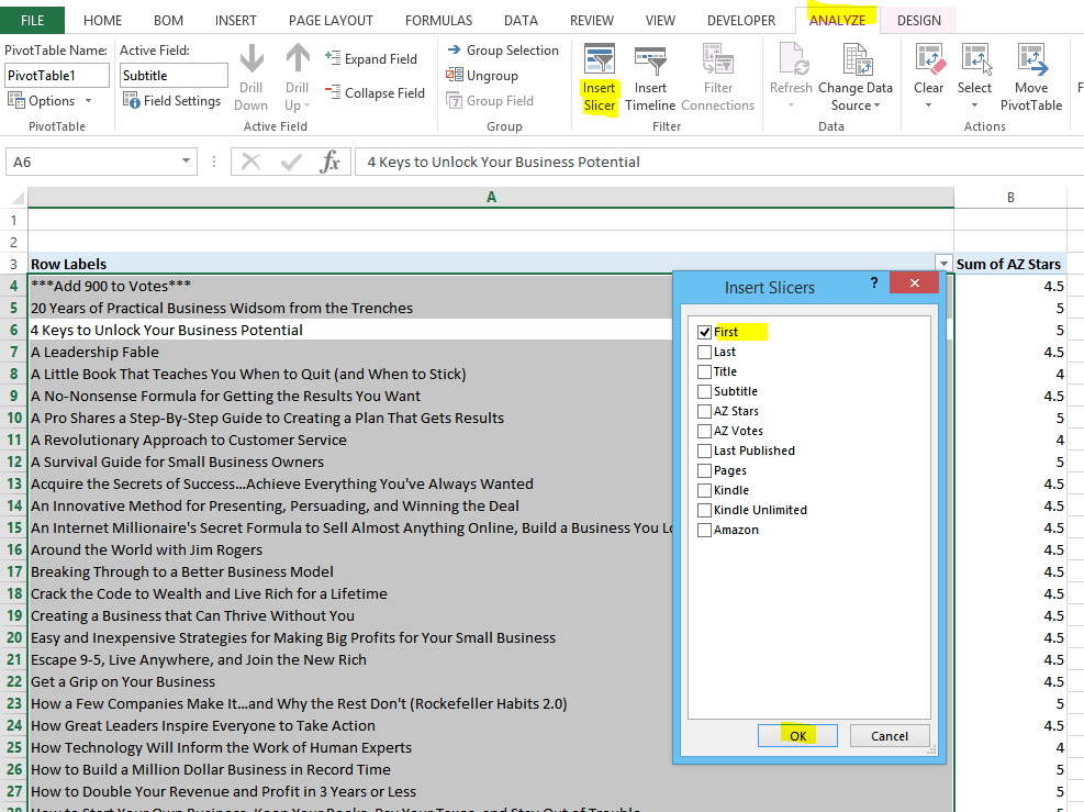
Instead of putting another entry in the "Filters" section of the pivot table, select the pivot table and press "Insert Slicer" in the "Analyze" tab. Then check out the field you want to filter:

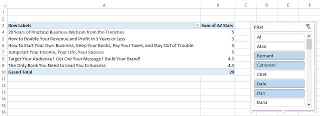
As a result you will have a user friendly menu where you can easily search for the name you want to filter and select multiple entry to sort out at once:

Created by DoMyExcel.com © | Excel & VBA Consulting | Customized Excel Solutions starting at 29 USD

Services provided to Individuals and Businesses | Free Quote: DoMyExcel@gmail.com

Excel Tip: Create a PivotTable of all the data in a sheet just by selecting one Cell.

A quick way of creating a PivotTable of the Data in one sheet is to select one of the cells that contains the data to Pivot. Excel will automatically select all the table and Pivot all the Data. 

In the example below only Cell C4 was selected. After clicking on PivotTable Excel automatically expanded the selection to be all the Data in Sheet 1.

Created by DoMyExcel.com © | Excel & VBA Consulting | Customized Excel Solutions starting at 29 USD

Services provided to Individuals and Businesses | Free Quote: DoMyExcel@gmail.com

How to highlight or hide error cells in an Excel pivot table

If you'd like not to show the error in a pivot table, simply go to the options and replace error by nothing:

Created by DoMyExcel.com © | Excel & VBA Consulting | Customized Excel Solutions starting at 29 USD

Services provided to Individuals and Businesses | Free Quote: DoMyExcel@gmail.com

How to group dates by months in an Excel pivot table

To display your dates by month in a pivot table, simply right click on the dates, press group and select both month and year:

Excel will automatically sum up your values and group them by months:

Created by DoMyExcel.com © | Excel & VBA Consulting | Customized Excel Solutions starting at 29 USD

Services provided to Individuals and Businesses | Free Quote: DoMyExcel@gmail.com

How to organize your data in Excel to make a pivot table

How to organize your data to easily create a consistent pivot chart

The easiest way to organize your data if you want to use the powerful tool of pivot chart in Excel is to work by columns with titles on first row, such as the example below:

 

Example: Planning / tracking of an entertainment company. The company tracks the number of ticket sold depending of the type of event (show / concert), the location of the event (main stage / second stage) and by date.

 

1) Organization of data base

Instead of presenting the database like this for example:

 

 

Pick up the different variables of the spreadsheet (type of event, location, number of ticket sold, date) and organize the database by columns, with the titles of the different variables in first row:

 

 

2) Pivot chart creation

Simply select the entire table and click on "Pivot Chart" (Menu "Insert").

 

 

Then locate the cell you want the pivot table to be created (Note that a pivot chart is always based on a pivot table).

 

3) Set up of the pivot chart

Example 1: Display the sum of tickets sold by type of event:

 

 

 

 

Example 2: Display the sum of tickets sold by stage and by type of event: 

 

 

 

Created by DoMyExcel.com

Customized Excel Solutions starting at $29!